1 Introduction to Posit, Rstudio, & Markdown
This week our goals are to be able to:
- Navigate the Posit and RStudio interface with proficiency.
- Articulate the process of using RStudio to develop markdown documents.
- Practice using markdown to format reproducible documents
1.1 Pre-work
- Read https://posit.cloud/learn/guide to learn a little bit about the Posit cloud space
- To get a quick intro to the Rstudio user interface
- watch this YouTube Video,
- or this one which is a little longer and provides some more motivation,
- or check out the Posit/Rstudio User Guide (if you prefer reading to videos).
- Check out the Posit/RStudio Introduction to Rmarkdown and Quarto
- Peruse the material below and complete week 1 concept check (in Canvas)
- Open the 01-2_Problem-Set.Rmd file from the files pane in the lower right and be ready to work through these materials on Monday.
1.2 Posit
Posit, the company, used to be called RStudio, but as they expanded beyond offering services just for R they decided to change their name. I thought that RStudio, the software, was also going to change names, because it is not just for working with R, but it hasn’t yet changed names. Posit now makes RStudio (which is still open source!) and also hosts RStudio servers via Posit.cloud that we pay for to help you all learn R, basic programming, data science, and engineering data analytics.
Within the Posit Cloud you will see “Spaces” to the left including the BSE 3144 workspace for this class. Within this workspace there are projects for each week. I can make “assignment” projects, which means that when you open the project it will make a copy of the project that you own and can edit and complete. Think about each of these new projects you make as your personal notebook for the class. Add your notes as you work through the material.
Within the project is the RStudio interface. This is just like if you installed R and RStudio on your computer only it is in a website. You can download R and RStudio on your computer if you like, following the directions at https://posit.co/download/rstudio-desktop/, but especially as we get deeper into the material installing packages can take a good chunk of time. By working in the environment we have set up for you in the Posit Cloud you can hopefully spend time learning in class or at home as opposed to setting up your computing environment. We will cover installing packages next week, and setting up your environment is a useful skill, but it is largely an exercise in patience, with the occasional internet troubleshooting/debugging (which we will cover in detail by week 03).
1.3 Rstudio
Rstudio (or Posit if they ever change it) is an integrated development environment, or IDE. An IDE is a program in which you can write code, view the outputs it creates, keep your code and outputs organized, and many other useful things. You can write R code in RStudio as well as many other programming languages. RStudio has lots of nice features. You can check out many of them by scanning through the menu bar. Tools>Global Options… also has many nice customization options including the the coveted hacker dark mode themes in the “Appearance” tab by changing the Editor Theme. A good IDE can make learning a language much easier, and even if you are an experienced coder a good IDE can make you much more efficient.
Let’s take a look around the RStudio window. You will see several panes within the RStudio window.
You will see several panes within the RStudio window.
1.3.1 The Source pane
If a file is open, in the top left of the screen perhaps this one, you will see the Source pane. (If you don’t see this pane, create a new file by pressing shift + command(or ctrl) + N, or click the universal ‘New Document’ icon  and select ‘R script’). Source shows the files with which you are currently working. This is where you will spend most of your time building and testing lines of code and then combining them to make scripts for data analysis. In general you should be doing most all of your typing into the source pane to build a document that you can use to reproduce your analysis.
In this class we will be mostly working in markdown documents in the source pane.
1.3.2 Markdown
Markdown is a document formatting computer language. The name markdown comes from html, or HyperText Markup Language, what websites are written in (along with a lot of other languages these days). Markdown is meant to be a much more chill version of html, but can also be used to make just about any kind of document from websites to PDFs, PowerPoint, and Word docxs. Markdown uses very simple text-based symbols to format text into potentially very attractive and useful documents.
Markdown is used in many different places these days, but we’ll use it in this class to help guide our data analyses. Remember: “If you are thinking without writing, you only think you are thinking!” -Leslie Lamport (emphasis my own). We will use markdown in the form of Rmarkdown or Quarto files. Rmarkdown is a product of Rstudio the company, and holding with the trend of changing names, the newest extended version of Rmarkdown is called Quarto, which really goes beyond R to include any programming language (or many at least). We will mostly use Rmarkdown in this class, for now, as most of the materials were developed before Quarto. But feel free to experiment with Quarto and I will do the same as I develop new materials.
When you make a new R Markdown document the following useful template begins the file.
1.3.2.1 R markdown
This is an R Markdown document. Markdown is a simple formatting syntax for authoring HTML, PDF, and MS Word documents. For more details on using R Markdown see http://rmarkdown.rstudio.com.
When you click the Knit button a document will be generated that includes both content as well as the output of any embedded R code chunks within the document. You can embed an R code chunk like this:
##      speed           dist
##  Min.   : 4.0   Min.   :  2.00
##  1st Qu.:12.0   1st Qu.: 26.00
##  Median :15.0   Median : 36.00
##  Mean   :15.4   Mean   : 42.98
##  3rd Qu.:19.0   3rd Qu.: 56.00
##  Max.   :25.0   Max.   :120.00
1.3.2.2 Including Plots
You can also embed plots, for example:
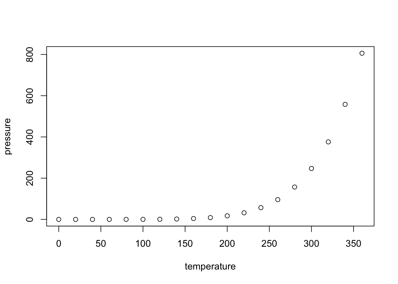
Note that the echo = FALSE parameter was added to the code chunk to prevent printing of the R code that generated the plot.
This provides a concise introduction to markdown and its power. Through simple text symbols your can format text to be headings (with #’s), make text bold, denote what is code, and offset code chunks with three back-ticks (the key next to 1 on your keyboard) and curly braces indicating the programming language. Code chunks (or blocks) also allow you to name them and changing some settings with how the code should be run and output.
Note how the above and all of this document (in its markdown format) has empty lines between text elements. This makes sure that particularly headings and sections, like numbered/bullet lists, are formatted correctly.
1.3.3 More Markdown formatting
There are lots of cool things you can do with markdown. Check out the resources available from links in the menu bar by going to Help>Markdown Quick Reference as well as Help>Cheat Sheets. There are cheat sheets for the RStudio IDE and a couple for R Markdown. We will practice with those a bit in Examples and your Problem Set.
You can also click “Visual” next to “Source” up at the top of this file to use a more traditional rich text format editor using mouse clicks to format your text. I have found this function is still a little glitchy and you especially need to be careful pasting text into the Visual editor.
There are some things the visual editor does make easier like inserting images and citations and formatting tables. As you’ll see below with the code chunk settings in Code chunk/block settings and global settings below.
Links and images are particularly useful for documents. You can link to any website you simply sandwich the text you want to be linked in square brackets, followed by parentheses containing the link/web-address/URL (uniform resource locator). Links can also be to sections (defined by headings in your document) as you see above (figuring out how the names change can be tricky though, I had to look in the knitted html file for the section above).
Images are similar but the link is the alt-text or caption text, and the link is a link or path to the image. The image can be somewhere in your project folder or anywhere on the internet. So for example we could use the code to insert this screenshot which is in this projects images folder:

For all file paths that you use in a markdown document the path is relative to the markdown document. So this Rmd is in the 01_Posit-Rstudio-Markdown folder and we only need to specify that, relative to this file, the screenshot above is in the images folder/directory and then we also need to specify the file name of the image.
1.3.4 Running code
Any line of code in a code chunk the source pane can be run in the Console pane by placing your cursor on that line and pressing control+enter (command+return on macs). Practice running the lines below in the code chunk.
## [1] 4## [1] 3## [1] 27## [1] FALSE## [1] TRUEThe result of the code is printed right below the chunk and is also shown in the Console pane below. You can also use the green play button (right-facing triangle) to run all of the lines in the chunk, or try to run either of the back-tick-containing top and bottom lines.
1.3.5 The Console pane
The Console pane is in the bottom-left corner labeled Console at the top left. (If the Source pane is closed, the Console pane may take up the whole left side of the window). The Console is essentially an R command line window. You can type in anything following the > then press return (or Enter) and whatever you typed will be interpreted by R and the appropriate output will be returned. R understands all basic algebra as well as logical expressions (aka Boolean expressions, such as 5<7 or True & False = False).
Most of the time you want to type your code into the source pane, but occasionally you will want to test something out or do a quick calculation that might not be needed in the file you are working on. Then you can work directly in the console.
In addition to being a basic calculator, R interprets functions or variables that can be assigned to and represented by words. Variables (any piece of data of any variety) will be single words possibly followed by a $ or square brackets [] if the variable is a matrix (a two dimensional array of data, where matrix$y would return column y and matrix[x,y] would return the piece of data in row x and column y). Functions (blocks of code that perform a specific function) are followed by parentheses containing the arguments/parameters on which that function will operate. For example, print("Hello World"), uses the print function to print the text argument (an argument is anything we pass to a function) “Hello World” if you run that line in the console.
Variables and Functions R is an object oriented language. This means we can use R to create abstracted objects that contain data (of any type, shape or size) called variables or procedures/methods (individual blocks of code) called functions. There are numerous functions and datasets included in the base R installation. Also, as an open source language countless programmers in the R community have written useful functions and created useful datasets that are freely available in the form of R-packages (more on these later). You can also write your own! But more on this in the
The big difference between using RStudio and running R from the command line is that this pane has an auto-complete feature. Try typing pri into the console below (or in a code chunk or Source pane and pressing tab. RStudio automatically provides you with a list of all the available functions and variables beginning with ‘pri’!
You can navigate this list using the arrow keys or your mouse. When you select a particular object, RStudio also gives you some information about that object. Navigate down to print (if there are multiple, select the one that has {base} at the far right) and press tab. You will see that RStudio has completed print in the console and added a set of parentheses because print is a function, print(). Now we can add arguments that this function will operate on, within the parentheses. But what does this function do? To figure out type ?print in the Console and press return. This opens the documentation for this function in the Help pane. A ? before any function name, or passing a function name to the help() function will do the same.
1.3.6 The Help pane
This pane is essentially a browser window for R documentation. You can also search for functions or variables in R and all of the installed packages on your computer using the search box at the top. You can search within a documentation page using the Find in Topic box.
Using this pane you should be able to answer almost any question you have about any R function.
All R documentation follows standard formatting. Description is pretty self explanatory. Usage demonstrates how you use the function, sometimes with specifics for different variable types. For print this shows us that print takes the input argument x (an argument is just variable that is used in a function). If x is a ‘factor’ or a ‘table’, print will also take some additional arguments. In the Usage section the default value of each argument is listed (e.g. FALSE is the default value for argument quote). A description of each argument is listed below in the Arguments section. Value is the type of data returned by the function. There are a few other self-explanatory sections and finally Examples. This is often one of the most useful sections as it shows you how to use the function. The code in Examples can be copied and pasted into the console and run.
1.3.7 The Files/Plots/Packages/Help/Viewer pane
The Help pane contains additional tabs that can also be quite helpful. Files allows you to navigate through folders on your computer and open files. Plots shows you the most recent plot your code has produced and allows you to save it. Packages allows you to install and load packages into memory. Packages are bundles of code that other people have written and shared with the community (more about packages later).
Additionally, there is a search engine specific to R resources including the documentation, blogs, books and questions users have asked on discussion boards. This invaluable resource is at Rseek.org. This is especially helpful if you want to find a function to perform a specific task.
1.3.8 OK, back to the Source pane…
You should have print() in there now.
Put your cursor in the middle of the parentheses and press tab. RStudio will feed you all of the arguments of this function using auto-complete! Press tab again and x = will appear in the parentheses. Type "hello world" and press command/ctrl + return/enter. This will copy your line of code into the console and execute it. Amazing! Your first line of R code worked, hopefully…
## [1] "hello world"Take note that if you are missing the quotes around hello world R will look for a variable named hello and return an error.
If your code didn’t work, try to fix it and run it again.
command + return (ctrl + enter on Windows machines) can be used to execute a whole line or any selected code.
Now just highlight x = "hello world" within the print(x = "hello world") line and press command + return (or ctrl + enter). This will just execute the highlighted text. If everything worked properly, you have just created your first variable object in R!
1.3.9 The Environment pane
See, over on the top right next to x (the variable object name) is “hello world” (the value assigned to that variable). You can now execute just print(x), and you will get [1] "hello world"! The Environment pane shows all of the objects you have created or stored in memory. You can view data sets or functions by clicking on them, but at the moment we only have the simple variable x. Don’t worry, we’ll practice this later.
1.3.10 The History/Connections/Git/Build/Tutorial pane
The Environment pane also has many tabs that can do lots of cool things. For now all that I want to cover is the History pane/tab. This keeps track of all of the code you have run. So if you forgot what you typed into the console, or you want to transfer something you ran in the Console into the Source pane, the History pane will do that for you.
1.3.11 Terminal/Render/Background Jobs
Also the Console pane has other tabs. Terminal can run Unix code. Render is for tracking markdown documents as they are rendering into whatever their output format is.
We are going to expand on using these panes and practice writing some more R code next week but for now we are going to focus a little more on R Markdown.
1.3.12 YAML headers
Each R Markdown or Quarto document starts with a YAML header like:
(Note if you are reading in markdown that I used a code chunk to make sure this header text didn’t mess up our current document).
YAML stands for Yet Another Markup Language and this header provides some data and variables or settings for how the document should be rendered, or knit.
We could change the YAML header of this document to make an HTML webpage version of this document for example by just changing
---
title: "01-0 Introduction to Posit, Rstudio, & Markdown"
author: "Clay Wright"
date: "2026-01-23"
output: pdf_document
---
to
---
title: "01-0 Introduction to Posit, Rstudio, & Markdown"
author: "Clay Wright"
date: "2026-01-23"
output: html_document
---
We could also make this into a docx or slides, but slides work a little differently. I made the slides on the first day of class in Quarto, you can check them out in that project.
In general this works quite well. But the YAML header is often a source of hard to track down errors. These errors can often be solved by replacing the header with the header from an RStudio template document.
1.3.13 Code chunk/block settings and global settings
Code chunk or block settings, which set how a code block will be run or formatted is one area in which R Markdown and Quarto differ.
(from https://www.stephaniehicks.com/jhustatprogramming2023/posts/2023-10-26-build-website/)
1.3.13.1 R Markdown vs Quarto
Some high-level differences include
- Standardized YAML across formats
- Decoupled from RStudio
- More consistent presentation across formats
- Tab Panels
- Code Highlighting
Another noticeable difference are settings/options for code blocks. Rather than being in the header of the code block, options are moved to within the code block using the #| (hash-pipe) for each line.
This is a code block for R Markdown:
(Note if you are reading in markdown that the text formatting is broken from here on. This is a known issue in RStudio https://community.rstudio.com/t/continued-issues-with-new-verbatim-in-rstudio/139737, and is possibly a reason to switch to Quarto).
This is a code block for Quarto:
1.3.14 Output Options
There are a wide variety of output options available for customizing output from executed code.
All of these options can be specified either
- globally (in the document front-matter) or
- per code-block
For example, here’s a modification of a Python-containing markdown example to specify that we don’t want to “echo” the code into the output document:
Note that we can override this option on a per code-block basis. For example:
Code block options available for customizing output include:
| Option | Description |
|---|---|
eval |
Evaluate the code chunk (if false, just echos the code into the output). |
echo |
Include the source code in output |
output |
Include the results of executing the code in the output (true, false, or asis to indicate that the output is raw markdown and should not have any of Quarto’s standard enclosing markdown). |
warning |
Include warnings in the output. |
error |
Include errors in the output (note that this implies that errors executing code will not halt processing of the document). |
include |
Catch all for preventing any output (code or results) from being included (e.g. include: false suppresses all output from the code block). |
Here’s a example with r code blocks and some of these additional options included:
---
title: "Knitr Document"
execute:
  echo: false
---
```{{r}}
#| warning: false

library(ggplot2)
ggplot(airquality, aes(Temp, Ozone)) +
  geom_point() +
  geom_smooth(method = "loess", se = FALSE)
```
```{{r}}
summary(airquality)
```
When using the Knitr engine, you can also use any of the available native options (e.g. collapse, tidy, comment, etc.) which help format your code chunks nicely in the final document.
See the Knitr options documentation for additional details. You can include these native options in option comment blocks as shown above, or on the same line as the {r} as shown in the Knitr documentation.
1.3.15 Troubleshooting Knit/Render problems
Knitting or Rendering markdown documents can lead to lots of tough to identify error messages. It is many of the questions we recieve. Especially right before assignments are due.
Here is a great write-up of common markdown problems: https://rmd4sci.njtierney.com/common-problems-with-rmarkdown-and-some-solutions.
Probably the most common issue we see is something (like your name in the author: line) in the YAML header that is not in quotes to indicate it is a string, or that there is some variable in your environment pane that is not actually created in your markdown document.
To avoid this second problem in the first place, I try and do the following:
- Develop code in chunks and execute the chunks until they work, then move on.
- knit the document regularly to check for errors.
Then, if there is an error:
- recreate the error in an interactive session:
- restart R
- run all chunks below
- find the chunk that did not work, fix until it does
- run all chunks below
- explore working directory issues
- remember that the RMarkdown directory is wherever the .Rmd file is in your Files pane